Low-Degree Extension

Articles based on Justin Thaler's Proofs, Arguments, and Zero-Knowledge

In the previous articles we performed Reed-Solomon encoding on various input vectors. The resulting encoded vectors were of length p which was a prime number much greater than the length of the original input, n. In this sense, we had created distance-amplified encodings which we used to construct some probabilistic procedures. These probabilistic procedures were more efficient than their deterministic counterparts.

Previously, we treated the values of the input vectors as coefficients to a univariate polynomial of degree n-1. It turns out that, in the context of interactive proofs and arguments of knowledge, it can actually be more useful to treat those values as evaluations of some polynomial rather than its coefficients.

From Coefficients to Evaluations

Lets illustrate the differences between treating our input elements as evaluations as opposed to coefficients of a polynomial with a simple worked example. Say we have an input vector a where n=4:

\(a=(0,1,2,0)\)

The Reed-Solomon encoding interprets a as the following polynomial:

\(p_a(x)=x+2x^2\)

Then we can achieve a distance amplified encoding of the original vector by evaluating its corresponding polynomial over a field of prime order p. In the past we mentioned that p should be a prime bigger than n², so lets say p=67. Then the Reed-Solomon encoding of a in Fp is:

\((0, 3, 10, 21, 36, 55, 11, ..., 1)\)

Now, if we instead treat a as evaluations of a univariate polynomial over some canonical input set, our encoded vector must look something like this:

\((0, 1, 2, 0, y_4, y_5,y_6,...,y_{66}) \)

Notice that the encoded vector is a superset of the input. As such, the encoding can be thought of as an extension of the input vector. Soon we will see that it is specifically a low-degree extension of a, or LDE(a),¹ and that low-degree extensions are actually more useful in the context of interactive proofs than our previous Reed-Solomon encodings. But how do we find this polynomial that corresponds to the evaluations found in LDE(a)? We do this through Lagrange interpolation.

Before we explain Lagrange interpolation, lets restate the context a little more formally. Paraphrasing lemma 2.3 from section 2.4 of Proofs, Arguments, and Zero-Knowledge: let p be a prime larger than n and Fp be the field of integers modulo p. For any vector a that is a subset of integers less than or equal to n in Fp, there is a unique univariate polynomial of degree at most n-1 such that:

\(q_a(i) = a_{i+1}\hspace{2mm} for \hspace{2mm} i = 0,...,n-1\)

This formula relates to the following definition of the input vector a:

\((a_1,...,a_n) \in \mathbb F^n\)

All that we are saying here is that there exists a unique univariate polynomial which, given some list of canonical inputs, evaluates to the values found in LDE(a).² We will show that this polynomial can be constructed as a linear combination of Lagrange basis polynomials. But first, we need to understand what a Lagrange basis polynomial is.

Univariate Lagrange Interpolation

In order to find the polynomial that evaluates the canonical input, (0,1,…,n-1), to LDE(a), we need to perform a linear combination of a set of Lagrange basis polynomials. We need a basis polynomial for every element in the canonical input.

Conceptually, a Lagrange basis polynomial is designed to map a single element of the canonical input to 1 and all others to 0. Specifically, the i’th Lagrange basis polynomial maps i to 1 and all other elements to 0. With that understanding, we can try digesting the following formula for Lagrange basis polynomials:

\(\delta_i(x)=\prod_{k=0,1,...,n-1\hspace{1mm}:\hspace{1mm}k\neq i} \frac{x-k}{i-k} \)

At face value it is probably unclear as to how this formula achieves the mapping we described above. For now, just trust that it does; when we go on to do the worked example, we will elaborate on this.

Next, we define our interpolated polynomial as the linear combination of the basis polynomials:

\(q_a(x)=\sum_{j=0}^{n-1} a_{j+1}\cdot\delta_j(x)\)

This simply means that the polynomial which evaluates each canonical input element to an element in LDE(a) is equivalent to the sum of all of our Lagrange basis polynomials weighted by their respective evaluations.³

Now lets do a simple worked example and build an intuition around why this makes sense. If n=4, then our basis polynomials behave as follows.

The first basis polynomial ensures that the evaluation is 1 when x=0. And that the evaluation is 0 when x is any of the remaining elements of the canonical input domain (1, 2, and 3).

\(\delta_0(x) = \frac{(x-1)\cdot(x-2)\cdot(x-3)}{(0-1)\cdot(0-2)\cdot(0-3)}\)

The second basis polynomial does the same for i=1.

\(\delta_1(x) = \frac{(x-0)\cdot(x-2)\cdot(x-3)}{(1-0)\cdot(1-2)\cdot(1-3)}\)

And the third and fourth basis polynomials do the same for i=2 and i=3, respectively.

Lets evaluate the fourth basis polynomial to make sure we understand whats going on here. When x=3:

\(\delta_3(3) = \frac{(3-0)\cdot(3-1)\cdot(3-2)}{(3-0)\cdot(3-1)\cdot(3-2)}\)

Obviously, when the numerator and denominator are equal and non-zero, the result is 1. This is the case whenever x=i , due to this part of the basis polynomial formula:

\(if\hspace{2mm}\frac{x-k}{i-k} =1, \hspace{2mm} then \hspace{2mm}x=i\)

Another way to put this is that the denominator normalizes the linear factor x-k. This normalization ensures that when all these terms are multiplied together, the resulting polynomial will evaluate to 1 when x=i.

When x is any element from the canonical input domain other than 3, say 1:

\(\delta_3(1) = \frac{(1-0)\cdot(1-1)\cdot(1-2)}{(1-0)\cdot(1-1)\cdot(1-2)} = \frac{1\cdot0\cdot-1}{1\cdot0\cdot-1}\)

Then the result must clearly be 0. This is because one of the n-1 factors in the equation will always evaluate to 0 when x is not the i’th element.

\(if\hspace{2mm}\frac{x-k}{i-k} =0, \hspace{2mm} then \hspace{2mm}x-k=0= i - k\)

So now we should have an intuition as to why basis polynomials evaluate to 1 and 0 when they need to. Here is a plot of the four basis polynomials:⁴

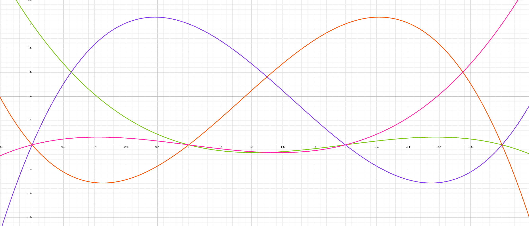
Notice that each x value that corresponds to an element in our canonical input relates to either a 0 or 1 y value. The next question you might ask is why a linear combination of the Lagrange basis polynomials results in the polynomial LDE(a).

Linear Combination of Basis Polynomials

Recall that the linear combination of the Lagrange basis polynomials is the sum of all the basis polynomials weighted by their respective evaluations. Lets break this out in our worked example from above, which involved the vector a=(0,1,2,0):⁵

\(q_a(x)=0\cdot \delta_0(x) + 1\cdot \delta_1(x) + 2\cdot \delta_2(x) + 0\cdot\delta_3(x)\)

This reduces to the following equation:

\(2^{-1}\cdot \:\:x\left(x-2\right)\left(x-3\right)\:-\:x\left(x-1\right)\left(x-3\right)\)

And if we plot this equation, it should look like an interpolation of our four basis polynomials:

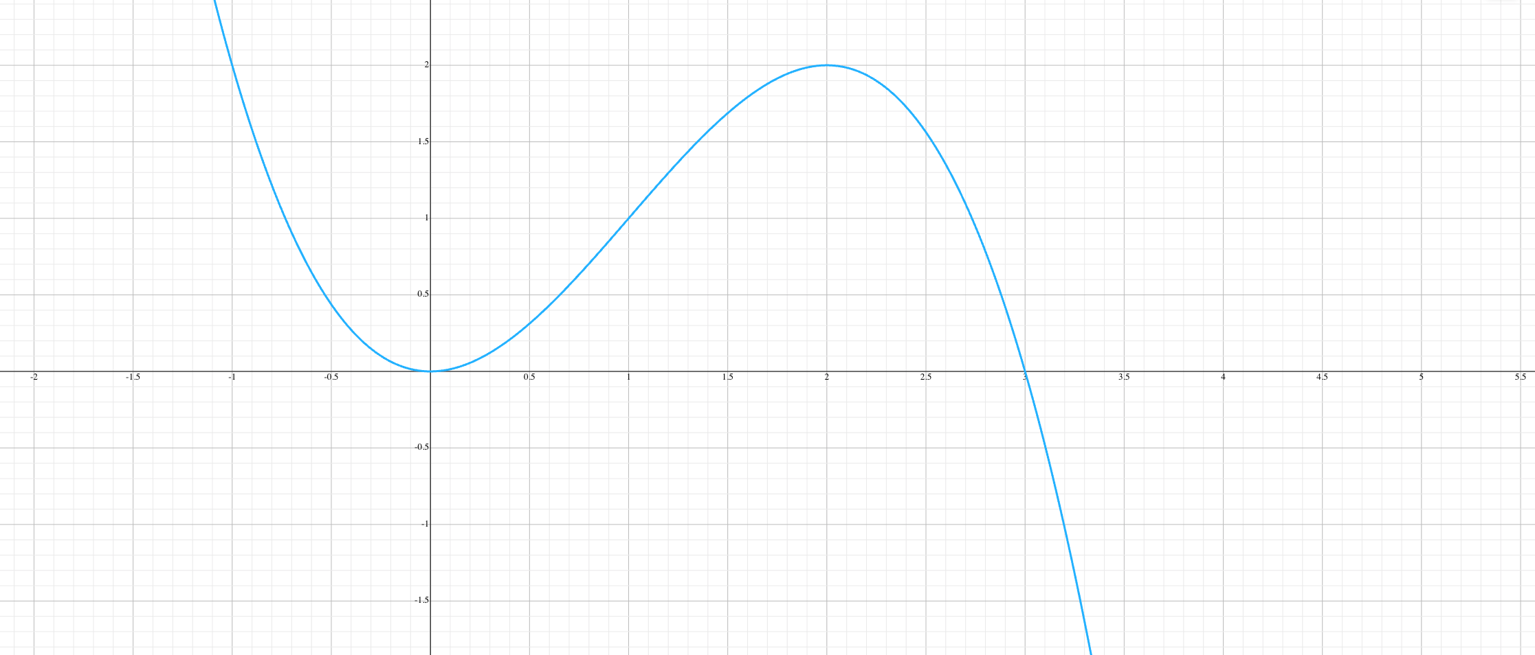
Take a moment to verify that this polynomial satisfies our LDE(a) which looks like this:

\((0, 1, 2, 0, y_4, y_5,y_6,...,y_{66})\)

While we can only verify the first four evaluations this way, we know that the interpolated polynomial is unique. Any two distinct polynomials of degree at most n-1 can agree on at most n-1 inputs. Since we created our polynomial from n inputs, there cannot be two distinct polynomials of degree at most n-1 that satisfy the equation.

If you are curious as to the full evaluation of LDE(a) or you want to walk through an educational implementation of the algorithm in Rust, you can use this. Running the relevant package will execute the worked example from above:

$ cargo run -p lagrange
    a = [0, 1, 2, 0]
LDE(a)= [0, 1, 2, 0, 59, 42, 13, 36, 41, ..., 2]

To conclude, we have used Lagrange interpolation to construct a low-degree extension of our n-sized vector a. The low-degree extension allows us to leverage those same probabilities we used in the previous articles with Reed-Solomon encoding due to the Schwartz-Zippel lemma. However, all of the techniques so far have resulted in polynomials of a maximum degree of n-1. This linear relationship between input size and polynomial degree is something that determines the utility of such techniques in the context of interactive proofs.

Multilinear Extension

In contrast to univariate low-degree extension which produces polynomials whose degree scales with input size, multilinear extension can produce polynomials whose total degree is logarithmic to the domain size. So, for example, if the domain of our elements is 2³², then the total degree of the multilinear extension is 32. Because their degree does not scale with input size, multivariate polynomials of ultra-low degree can be more practical than their univariate counterparts for various use cases.

We will explore multilinear extension and other techniques involved in interactive proofs in future articles.

1. In this article we will use LDE(a) to refer to both the interpolated polynomial as well as the vector containing all possible evaluations of that polynomial over the finite field.

2. The set of canonical inputs here is (0,1,…,n-1).

3. Remember that the evaluations are the elements in vector a.

4. Note that the graph is over the set of real numbers whereas the domain we are interested in is Fp.

5. Remember that the vector a is also a subset of LDE(a). Namely, the first n elements.

---

Artwork by fullvector from Freepik.